Neural Networks

1. Introduction to Neural Networks

Artificial Neural Networks (ANNs) are a class of machine learning models inspired by the human brain. Just like the brain is composed of interconnected neurons, ANNs consist of interconnected artificial neurons (also called nodes or units) organized into layers. Each artificial neuron receives input signals, processes them, and produces an output signal that can be passed to other neurons. The connections between neurons have weights that determine how much one neuron's output will affect another. By adjusting these weights, the network can learn to perform useful tasks such as classification, regression, and pattern recognition.

Imagine teaching a computer to distinguish between pictures of cats and dogs, translate languages in real-time, or predict stock market trends. Neural networks are the core technology behind these advances, providing a powerful way to learn complex patterns from data without being explicitly programmed with rules.

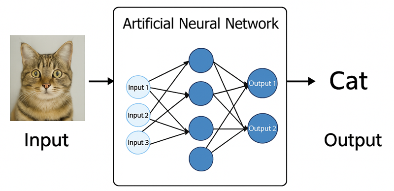
그림 1.1: 신경망의 기본 역할을 보여주는 다이어그램. 왼쪽에는 입력(예: 고양이 이미지). 가운데에는 "인공 신경망"이라고 표시된 상자. 오른쪽에는 출력(예: "고양이"라는 텍스트 레이블).

Neural networks are powerful because they can learn from data. Through a training process, an ANN can adjust its weights based on errors made in predictions, gradually improving its performance. In modern practice, most neural networks are trained using an algorithm called backpropagation together with an optimization method such as gradient descent. This allows even multi-layer networks to learn complex patterns by iteratively reducing the difference between the network's predictions and the true targets. It's important to remember that the brain analogy is a loose one; an artificial neuron is a powerful mathematical abstraction, but it is an extreme simplification of a complex biological neuron.

2. The Perceptron: A Single Neuron

The Perceptron is the simplest type of artificial neuron and the fundamental building block of neural networks. It's a model that takes several binary inputs and produces a single binary output. Understanding its simple mechanism is key to understanding more complex networks.

The Perceptron's Calculation Flow

A perceptron works by following a clear, step-by-step process to make a decision:

Receive Inputs: It starts with a set of input values, $x_1, x_2, \dots, x_n$.
Compute Weighted Sum: Each input $x_i$ is multiplied by a corresponding weight $w_i$. The weights signify the importance of each input. All these weighted inputs are summed up, along with a bias term $b$, to produce a single value, $z$. The bias can be thought of as a "thumb on the scale," making it easier or harder for the neuron to fire.
Apply Activation Function: The weighted sum $z$ is then passed through an activation function. In a classic perceptron, this is a simple "step function" that outputs 1 if the input $z$ is above a certain threshold (usually 0), and 0 otherwise.
Produce Output: The result from the activation function is the final output, $y$, of the perceptron.

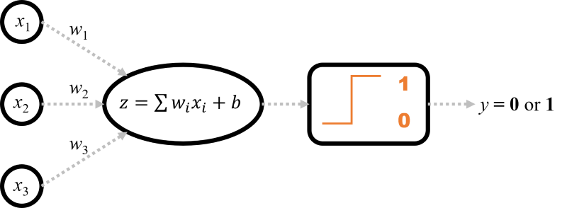
그림 2.1: 퍼셉트론 구조의 순서도. 입력(x1, x2, x3)이 중앙 노드로 들어갑니다. 각 연결에는 가중치(w1, w2, w3)가 표시되어 있습니다. 노드 내부에는 "가중 합계: z = Σ(wᵢxᵢ) + b"가 표시되고, 이는 "활성화(계단 함수)"를 가리키며 최종적으로 "출력 y (0 또는 1)"로 이어집니다.

A Concrete Example: The AND Gate

Let's see how a perceptron can represent a simple logical AND gate. The AND gate outputs 1 only if both of its inputs are 1.

Let's manually set the weights and bias to solve this problem: let $w_1 = 1$, $w_2 = 1$, and $b = -1.5$. The perceptron's decision rule is to output 1 if $z = (1 \cdot x_1) + (1 \cdot x_2) - 1.5 > 0$, and 0 otherwise.

For input (1, 1): $z = (1 \cdot 1) + (1 \cdot 1) - 1.5 = 0.5$. Since $0.5 > 0$, the output is 1. (Correct)
For input (1, 0): $z = (1 \cdot 1) + (1 \cdot 0) - 1.5 = -0.5$. Since $-0.5 \le 0$, the output is 0. (Correct)
For input (0, 0): $z = (1 \cdot 0) + (1 \cdot 0) - 1.5 = -1.5$. Since $-1.5 \le 0$, the output is 0. (Correct)

This simple example shows that with the right weights and bias, a single perceptron can model a basic logical function.

Visualizing the Decision Boundary

The parameters $w_1, w_2, \dots$ and $b$ that the perceptron learns are not just abstract numbers; they define a **linear decision boundary**. For a 2D problem like the AND gate, this boundary is a straight line. The equation of this line is $w_1x_1 + w_2x_2 + b = 0$. All points on one side of the line are classified as one class (e.g., 1), and all points on the other side are classified as the other class (e.g., 0).

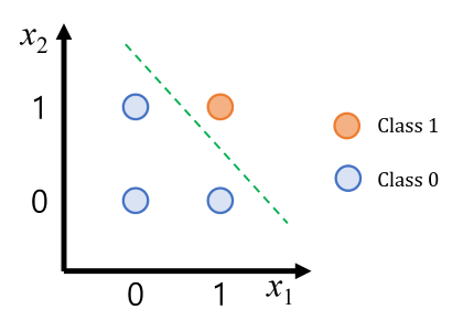
그림 2.2: AND 게이트의 결정 경계를 보여주는 2D 그림. 점 (0,0), (0,1), (1,0)은 클래스 0으로, 점 (1,1)은 클래스 1로 색칠되어 있습니다. 그림에는 직선이 그려져 있어 점 (1,1)이 다른 세 점과 명확하게 구분됩니다.

Geometrically, the weight vector $\vec{w} = (w_1, w_2)$ is always perpendicular (orthogonal) to the decision boundary line. The magnitude of the weights affects the slope, and the bias $b$ shifts the line away from the origin. This geometric view is crucial for understanding why a single perceptron can only solve problems where the classes can be separated by a single straight line.

How a Perceptron Learns

So how does a perceptron find the correct weights and bias automatically? It uses a simple iterative process called the **Perceptron Learning Algorithm**:

Initialize: Start with random values for weights and bias.
Iterate: For each training example:
1. Make a prediction using the current weights.
2. Compare the prediction ($\hat{y}$) with the true label ($y$).
3. If the prediction is wrong, update the weights and bias to correct the mistake.
Repeat: Continue this process until the perceptron makes no more mistakes on the training data.

The update rule is simple and intuitive. For each weight $w_i$, the update is: $ w_i(\text{new}) \leftarrow w_i(\text{old}) + \eta \cdot (y - \hat{y}) \cdot x_i $. The term $\eta$ (eta) is the learning rate, a small number that controls the step size of the update. If the prediction is correct, $(y - \hat{y}) = 0$ and no update occurs. If it's wrong, the weights are nudged in the direction that would bring the prediction closer to the true label.

3. Limitation of a Single Neuron: The XOR Problem

A single perceptron has significant limitations. It can only learn to classify data that is linearly separable—meaning a single straight line (in 2D) or hyperplane (in higher dimensions) can separate the classes. Many problems in the real world are not linearly separable. A classic example is the XOR logic function.

XOR (short for "exclusive OR") takes two binary inputs and returns 1 if exactly one of the inputs is 1, and returns 0 otherwise.

XOR Truth Table
Inputs (A, B)	Output
(0, 0)	0
(0, 1)	1
(1, 0)	1
(1, 1)	0

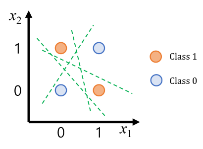
XOR 데이터 포인트 네 개를 그린 그림으로, 하나의 직선으로는 분리할 수 없음을 보여줍니다. (0,0)과 (1,1)은 한 가지 색으로, (0,1)과 (1,0)은 다른 색으로 표시되어 있습니다.

If we plot these input pairs, it's visually clear there is no single straight line that can separate the '0' class from the '1' class. Because the XOR data is not linearly separable, a single-layer perceptron cannot solve XOR. This limitation motivates the need for multiple neurons and layers.

4. From Perceptron to Multi-Layer Perceptrons (MLPs)

The solution to non-linear problems is to use multiple neurons working together in what's called a Multi-Layer Perceptron (MLP). An MLP is a type of feedforward neural network that has an input layer, one or more hidden layers, and an output layer. While a single perceptron can only draw one line, an MLP can create much more complex, non-linear decision boundaries.

The power of the MLP comes from its hidden layers. Think of it this way: each neuron in the first hidden layer learns to draw its own simple line. The next layer can then learn to combine the outputs of the first layer, effectively combining their lines to form more complex shapes (like corners, circles, or enclosed regions). The final output layer then makes a decision based on these complex, learned features. This is how an MLP can solve a problem like XOR—by using multiple lines to isolate the correct regions of the data.

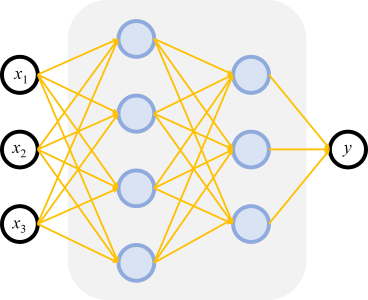
그림 4.1: 입력층, 은닉층, 출력층으로 구성된 MLP의 기본 아키텍처를 보여주는 다이어그램. 각 층의 노드는 다음 층의 노드와 완전히 연결되어 있습니다.

Mathematical Foundations

In an MLP, data flows forward from the input layer to the output layer. The operation in the l-th layer is expressed in matrix form as follows, where the input is the activation output from the previous layer, $A^{[l-1]}$:

$$ Z^{[l]} = W^{[l]}A^{[l-1]} + b^{[l]} $$ $$ A^{[l]} = g^{[l]}(Z^{[l]}) $$

$W^{[l]}$: Weight Matrix
$b^{[l]}$: Bias Vector
$Z^{[l]}$: Linear Output
$g^{[l]}$: Activation Function
$A^{[l]}$: Activation Output of the l-th layer

The Role of Activation Functions

The activation function introduces non-linearity, which is a crucial feature. Without a non-linear activation function, an MLP with any number of layers would be mathematically equivalent to a single-layer perceptron. It is the non-linearity that allows the network to learn complex relationships far beyond simple lines. It's the key that unlocks the "deep" in deep learning.

그림 4.2: MLP가 XOR 문제를 어떻게 해결하는지 보여주는 개념도. 한 패널에는 은닉층 뉴런에 의해 그려진 두 개의 선이 표시됩니다. 두 번째 패널에서는 이러한 선들이 결합되어 XOR 점들을 올바르게 분리하는 비선형 경계를 만드는 방법을 보여줍니다.

Function	Equation	Key Characteristics
Sigmoid	$\sigma(z) = \frac{1}{1+e^{-z}}$	Outputs a value between 0 and 1. Historically used but prone to vanishing gradients.
Tanh	$\tanh(z) = \frac{e^z - e^{-z}}{e^z + e^{-z}}$	Similar shape to sigmoid but zero-centered, with a range from -1 to 1.
ReLU	$\text{ReLU}(z) = \max(0, z)$	Very popular in modern networks for its simplicity and effectiveness in mitigating vanishing gradients. Outputs 0 for negative inputs and is linear for positive inputs.

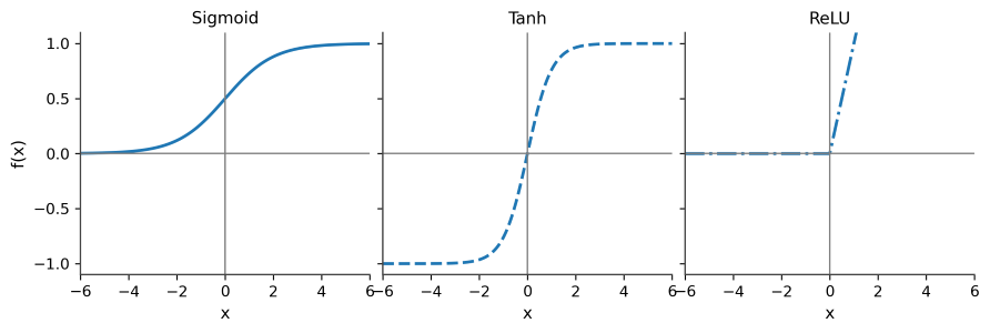
그림 4.3: 시그모이드, Tanh, ReLU 활성화 함수의 그래프를 나란히 보여주어 쉽게 비교할 수 있는 그림.

Hard step functions are rarely used in hidden layers of trainable networks now because they are not differentiable, which makes learning with gradient-based methods difficult.

5. The Training Process

Training a neural network means finding the weights and biases for all neurons that make the network perform well on a given task. This typically involves supervised learning, where we have a dataset of examples with known correct outputs (labels).

Loss Function

To quantify how well the network is doing, we define a loss function (also called a cost function). The loss is a single number that is high when the network's predictions are poor and low when predictions are accurate.

Mean Squared Error (MSE): Used for regression. $J = \frac{1}{m}\sum_{i=1}^{m}(\hat{y}^{(i)} - y^{(i)})^2$
Cross-Entropy: Used for classification. For binary classification, the loss is $J = -\frac{1}{m}\sum_{i=1}^{m}[y^{(i)}\log(\hat{y}^{(i)}) + (1-y^{(i)})\log(1-\hat{y}^{(i)})]$

Gradient Descent and Backpropagation

This is conceptually the most challenging part of deep learning, but it can be understood with a powerful analogy: finding the lowest point in a mountain range while blindfolded.

The Loss Function is the mountainous terrain. The altitude at any point represents the model's error (or loss). High altitude means high error.
Your model's current weights and biases define your position (latitude and longitude) on this terrain.
The Goal is to find the lowest valley (the point of minimum loss).
Gradient Descent is your strategy. At your current position, you feel the ground around you to find the direction of the steepest slope downward (this is the negative gradient). You then take a small step in that direction.
The Learning Rate ($\eta$) is the size of your step. Too large, and you might overshoot the valley entirely. Too small, and it could take forever to get to the bottom.
Backpropagation is the "magic" that allows this to work for millions of weights. It is a highly efficient algorithm (based on the chain rule from calculus) that calculates the exact contribution of every single weight to the final error. In our analogy, it's the magical GPS that instantly tells you the steepest downhill direction, no matter how complex the terrain or how many dimensions you're in.

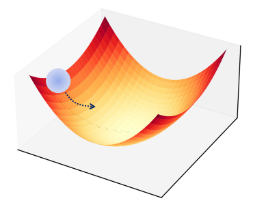
그림 5.1: 손실 함수를 나타내는 3D 표면 그림. 공이 높은 지점에서 시작하여 화살표로 표시된 경로를 따라 표면의 가장 낮은 지점(전역 최솟값)으로 굴러가는 모습이 보입니다.

Neural networks are typically trained by an iterative optimization process called gradient descent. The general idea is to update weights in the opposite direction of the gradient of the loss function. The update rule is: $w \leftarrow w - \eta \frac{\partial L}{\partial w}$, where $\eta$ is the learning rate.

The key algorithm that makes this feasible for multi-layer networks is Backpropagation. Backpropagation is how we efficiently compute the gradient of the loss with respect to all weights in a network. It works by applying the chain rule of calculus systematically, propagating error sensitivities backward from the output layer through the network.

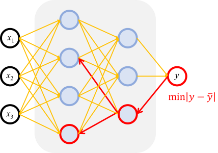
그림 5.2: 훈련 흐름을 설명하는 다이어그램. "순방향 전파"라고 표시된 화살표는 데이터가 입력에서 출력으로 이동하여 예측을 생성하는 것을 보여줍니다. 오차가 계산된 다음, "역방향 전파(역전파)"라고 표시된 새 화살표는 오차 신호가 출력에서 입력으로 역방향으로 흐르며 그 과정에서 가중치를 업데이트하는 것을 보여줍니다.

Advanced Optimizers and Regularization

In practice, we often use more advanced optimizers that build on standard gradient descent, such as Adam (Adaptive Moment Estimation), which adaptively tunes the learning rate for each weight and includes momentum terms. To train high-performing models, preventing overfitting and stabilizing the training process is essential. This is achieved through regularization techniques.

L1/L2 Regularization (Weight Decay): Adds a penalty term for large weights to the loss function, reducing model complexity.
Dropout: During training, randomly sets a fraction of input units to 0 at each update. This forces the model to learn more robust features. Think of it like training a large team for a project, but for every task, you randomly ask some members to sit out. This prevents the team from becoming overly reliant on a few "star" members and forces everyone to be competent. The result is a more robust and versatile final team (model).
Early Stopping: Monitors the loss on a validation set and halts training when the validation loss stops improving, preventing overfitting.
Batch Normalization: Normalizes the inputs to a layer for each mini-batch, leading to a more stable and faster training process.

6. Practical Implementation in Python

6.1 Solving XOR with Scikit-learn

To make the concepts concrete, we can solve the XOR problem with a small neural network using Python. We will use scikit-learn's MLPClassifier. Note that training can be sensitive to hyperparameters; the settings below are chosen to be robust and lead to a correct solution reliably.

When you run this code, you will see that the single-layer Perceptron fails to learn the XOR function, as expected. In contrast, the two-layer MLP with these more robust settings successfully learns to predict the correct XOR outputs `[0 1 1 0]`, demonstrating that the hidden layer enables the network to solve a problem that a single neuron could not.

6.2 Advanced Implementation with TensorFlow/Keras

For more complex problems, professional deep learning frameworks like TensorFlow are used. Below is an example of building an image classification model.

7. Lab: Electrochemical Applications

Neural networks excel at modeling the complex, non-linear relationships inherent in electrochemical data. This section provides three practical, hands-on examples that demonstrate how to apply NNs to common electrochemical problems.

7.1 Example 1: Classifying CV Data (Classification)

Problem: The shape of a Cyclic Voltammogram (CV) provides a fingerprint of the underlying electrochemical mechanism. We will train a network to classify a CV curve as belonging to a Reversible (E), **Irreversible (EC)**, or **Catalytic (EC')** mechanism.

Approach: We use a realistic, pre-defined dataset that captures the distinct features of these three mechanisms. The network will take the current values of the CV as input and perform a 3-class classification.

7.2 Example 2: Parameter Extraction from EIS Data (Regression)

Problem: Extracting physical parameters from Electrochemical Impedance Spectroscopy (EIS) often requires complex non-linear curve fitting. We will train an NN to directly predict the parameters of a Randles circuit ($R_s, R_{ct}, Q$) from a raw impedance spectrum.

7.3 Example 3: Predicting Battery Capacity Fade (Predictive Modeling)

Problem: Predicting the long-term performance and Remaining Useful Life (RUL) of batteries is critical. We will train a network to predict the capacity of a battery at a late cycle (e.g., cycle 500) using features from early cycles (e.g., cycle 10).

8. Conclusion and Next Steps

We have introduced the fundamental ideas of neural networks, from the Perceptron to Multi-Layer Perceptrons, which form the basis of modern deep learning.

Key Takeaways:

A perceptron is a single artificial neuron that can classify linearly separable data by finding a linear decision boundary.
A single perceptron cannot solve problems that are not linearly separable, like the XOR problem.
By adding hidden layers to form an MLP, we can solve much more complex tasks. The hidden layers enable the network to create non-linear decision boundaries.
Non-linear activation functions are vital for the power of MLPs.
Neural networks learn by using an optimization algorithm like gradient descent to minimize a loss function, with gradients computed efficiently by backpropagation.

From here, you are prepared to explore more advanced topics:

Other Architectures: There are specialized networks for different data types.
- Convolutional Neural Networks (CNNs) are used for image data.
- Recurrent Neural Networks (RNNs) are used for sequence data like time series or text.
Practical Considerations: Learn about preventing overfitting, choosing hyperparameters, and determining how much data is needed.

All advanced topics build on the core ideas you've learned here: weighted sums, activation functions, and iterative training via backpropagation.

Function	Equation	Key Characteristics
Sigmoid	\(\sigma(z) = \frac{1}{1+e^{-z}}\)	Outputs a value between 0 and 1. Historically used but prone to vanishing gradients.
Tanh	\(\tanh(z) = \frac{e^z - e^{-z}}{e^z + e^{-z}}\)	Similar shape to sigmoid but zero-centered, with a range from -1 to 1.
ReLU	\(\text{ReLU}(z) = \max(0, z)\)	Very popular in modern networks for its simplicity and effectiveness in mitigating vanishing gradients. Outputs 0 for negative inputs and is linear for positive inputs.