1. Introduction to Convolutional Neural Networks
Convolutional Neural Networks (CNNs or ConvNets) are a specialized class of neural networks designed to process data with a grid-like topology, such as an image. An image can be seen as a 2D grid of pixels, and CNNs are engineered to effectively capture the spatial relationships and hierarchies of features within this grid. Inspired by the organization of the animal visual cortex, CNNs have revolutionized the field of computer vision, achieving state-of-the-art results in tasks like image classification, object detection, and semantic segmentation.
1.1 How CNNs "See": Receptive Fields and Spatial Hierarchy
Unlike a standard Multi-Layer Perceptron (MLP), a CNN does not process an image all at once. Instead, it uses a small filter (or kernel) that scans the image in small patches. The specific region of the input that a filter looks at to compute a single value in the output feature map is called the receptive field. Early layers in a CNN have small receptive fields, allowing them to recognize fundamental patterns like edges, corners, or specific colors.
This is the foundation of CNN's ability to learn a spatial hierarchy. Here’s how it works:
- Layer 1: A filter with a small receptive field detects simple edges and color gradients.
- Layer 2: This layer doesn't see the original image, but rather the feature maps from Layer 1 (maps of where edges/colors are). Its filters combine these simple patterns into more complex shapes like textures, circles, or squares.
- Deeper Layers: This process continues, with each subsequent layer having a larger effective receptive field. They learn to combine the shapes from the previous layer into even more complex concepts, such as an eye, a nose, or a car's wheel, eventually leading to the recognition of the entire object.
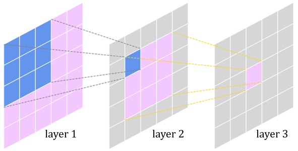
A visualization of how a receptive field in a deeper layer corresponds to a larger area of the original input image, showcasing the learning of a spatial hierarchy.
1.2 Key Hyperparameters: Stride and Padding
The behavior of the convolution operation is controlled by two key hyperparameters: stride and padding.
- Stride: This parameter defines how many pixels the filter moves at each step as it slides across the input. A stride of 1 means the filter moves one pixel at a time, creating a densely populated feature map. A larger stride (e.g., 2) causes the filter to skip pixels, resulting in a smaller output feature map, reduced computational cost, and a form of downsampling.
- Padding: This involves adding extra pixels (usually with a value of zero) around the border of the input image before the convolution. Padding serves two main purposes:
- Preserving Feature Map Size: Without padding, feature maps would shrink after every convolution. By adding padding, we can control the output dimensions, often keeping them the same as the input.
- Improving Edge Detection: Pixels at the image's border are covered by the filter fewer times than pixels in the center. Padding ensures these edge pixels get more robustly processed, improving the quality of feature extraction at the boundaries.
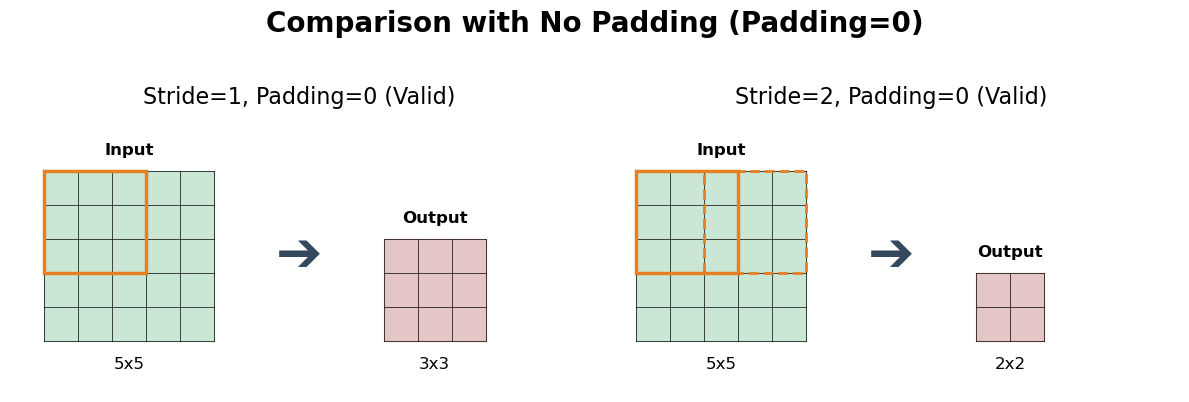
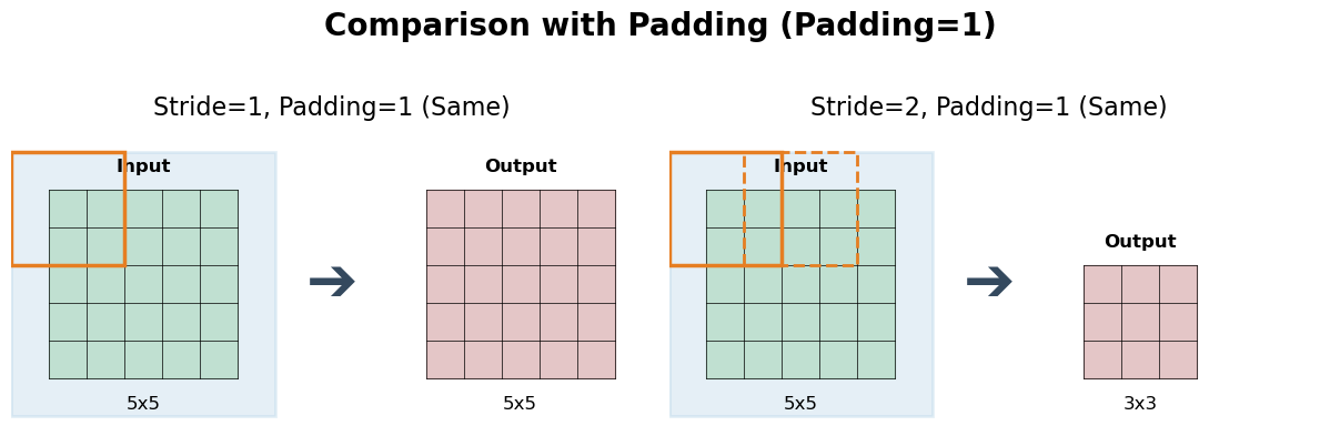
A comparison showing how different stride and padding settings (e.g., Stride=1 vs. Stride=2, No Padding vs. Same Padding) affect the final size of the output feature map.
2. The Problem with Fully Connected Networks for Images
While a Multi-Layer Perceptron (MLP) can theoretically be used for image classification, it is fundamentally ill-suited for the task due to three critical issues: massive parameter counts, loss of spatial information, and high computational cost.
2.1 The Parameter Explosion
An MLP requires every input pixel to be connected to every neuron in the first hidden layer. This leads to an unmanageable number of parameters as image size increases.
- For a tiny 32x32x3 color image, the input vector has 3,072 features. A single hidden layer with 1000 neurons would already require 3,072 × 1,000 = over 3 million parameters.
- For a standard 224x224x3 color image, the input vector size is 150,528. The same hidden layer would now require 150,528 × 1,000 = over 150 million parameters. A deep MLP would easily reach billions of parameters.
This "parameter explosion" makes the model incredibly slow to train, memory-intensive, and extremely prone to overfitting, as the model has too much capacity for the amount of data it typically sees.
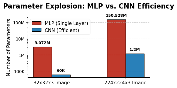
A bar chart showing the exponential growth in parameters for an MLP vs. the efficiency of a CNN when handling 32x32 and 224x224 images.
2.2 Loss of Spatial Information
To feed an image to an MLP, we must "flatten" the 2D grid of pixels into a 1D vector. This process destroys the image's inherent spatial structure. Pixels that were originally close together (e.g., forming an edge) are treated no differently from pixels that were far apart. The model loses all information about the arrangement of features, making it very difficult to learn concepts like shapes, textures, or object parts.
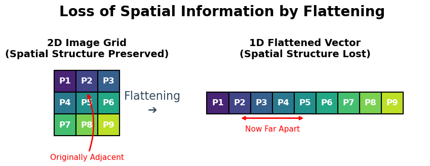
A simple graphic showing a 3x3 grid of pixels being flattened into a 9x1 vector, demonstrating that the spatial relationship between pixels is lost.
In contrast, CNNs use convolutional filters that explicitly operate on local neighborhoods of pixels, preserving and leveraging this spatial information. This makes them far more efficient and effective for image-based tasks.
3. The Core Components of a CNN
A CNN is built from a sequence of layers. While the convolutional layer is the star, several other components are essential for building a high-performing network.
3.1 The Convolutional Layer
This is the primary building block of a CNN. It uses a set of learnable filters (kernels) to detect features. A filter is a small matrix of weights that slides (or "convolves") across the input. At each position, it computes a dot product between the filter and the input pixels it covers, creating a single value in an output "feature map."
The core principles are:
- Local Connectivity: Neurons are only connected to a small, local region of the input (the receptive field).
- Parameter Sharing: The same filter (set of weights) is used across the entire input image. This allows the network to detect a feature (e.g., a vertical edge) regardless of its position, making the model translation invariant and drastically reducing the total number of parameters.
A 3x3 filter scanning an input matrix to generate a feature map, highlighting the element-wise multiplication and sum.
3.2 The Activation Function (Introducing Non-Linearity)
After each convolution operation, an activation function is applied element-wise to the feature map. Without it, the entire network would just be a series of linear operations, making it equivalent to a single, much simpler linear model. The activation function introduces non-linearity, allowing the network to learn complex patterns.
The most common activation function in CNNs is the Rectified Linear Unit (ReLU). It is defined as $f(x) = \max(0, x)$. It simply converts all negative values to zero. This makes the network easier and faster to train and helps mitigate the vanishing gradient problem. A common variant is Leaky ReLU, which allows a small, non-zero gradient for negative inputs to prevent "dying neurons."
3.3 The Pooling Layer (Downsampling)
A pooling (or subsampling) layer is often placed after the activation function. Its purpose is to progressively reduce the spatial size (width and height) of the representation. This has two key benefits:
- It reduces the number of parameters and computational complexity.
- It provides a degree of translation invariance, making the model more robust to the exact position of features.
Common types of pooling include:
- Max Pooling: The most popular choice. It takes the maximum value from a small rectangular window (e.g., 2x2) at each step. This effectively reports the most activated feature in the patch.
- Average Pooling: Takes the average value from the window instead of the maximum. It provides a smoother downsampling.
- Global Pooling (e.g., Global Average Pooling): A more extreme form where the entire feature map is reduced to a single value (its average or maximum). This is often used at the end of the network to drastically reduce parameters before the final classification layer.
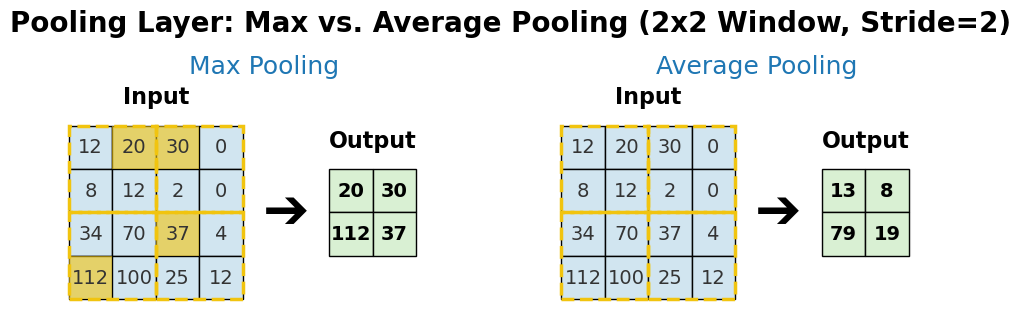
A side-by-side comparison showing how a 2x2 Max Pooling and a 2x2 Average Pooling operation produce different results on the same input feature map.
3.4 Regularization for Stability and Overfitting
Deep neural networks are prone to overfitting. Regularization techniques are crucial for building robust models that generalize well to new data.
- Batch Normalization: This technique normalizes the output of a previous layer by re-centering and re-scaling it. It is typically applied after the convolution and before the activation function. Batch Norm helps stabilize and accelerate the training process by reducing "internal covariate shift," allowing for higher learning rates.
- Dropout: A simple yet powerful technique where, during training, a random fraction of neurons are temporarily "dropped" (ignored) at each update step. This prevents neurons from co-adapting too much and forces the network to learn more robust and redundant features.
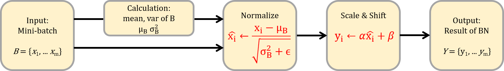
Flowchart of Batch Normalization: A diagram showing a mini-batch of activations being normalized (mean subtracted, divided by standard deviation) before being passed to the next layer.
3.5 The Fully Connected (Dense) Layer
After several convolutional and pooling layers have extracted a rich set of spatial features, the final feature maps are "flattened" into a 1D vector. This vector is then fed into one or more standard fully connected layers (an MLP), just like in a basic neural network. This part of the network acts as a classifier, using the high-level features to make the final prediction (e.g., assigning probabilities to each class).
4. Assembling a Full CNN Architecture
A typical CNN architecture stacks layers sequentially. A common pattern is:
INPUT → [CONV → (BN) → RELU → POOL] × N → FLATTEN → [FC → RELU] × M → OUTPUT
While early models like LeNet-5 and AlexNet followed this simple pattern, modern architectures like VGG, ResNet, and MobileNet introduce more sophisticated building blocks to improve performance and efficiency.
4.1 Advanced Architectural Blocks
Residual Connections (ResNet)
As networks get deeper, they suffer from the vanishing gradient problem, making them difficult to train. The groundbreaking idea behind ResNet is the "residual connection" or "skip connection." Instead of forcing a set of layers to learn a target mapping $H(x)$, we let them learn the residual mapping $F(x) = H(x) - x$. The original mapping is then reformulated as $F(x) + x$.
This is implemented as a "shortcut" that skips one or more layers and adds the input $x$ directly to the output of the convolutional block. This has two major benefits:
- Improved Gradient Flow: The skip connection provides a direct path for the gradient to backpropagate, mitigating the vanishing gradient problem and allowing for the training of extremely deep networks (over 100 layers).
- Easier Identity Mapping: If a layer is not needed, the network can easily learn to make the residual $F(x)$ zero, effectively turning the block into an identity mapping ($H(x)=x$). This means adding more layers is less likely to harm performance.

A diagram showing an input 'x' that passes through a block of layers (Conv -> BN -> ReLU -> Conv -> BN) to produce F(x). The original input 'x' is then added to F(x) before the final ReLU activation.
Depthwise Separable Convolutions (MobileNet)
Standard convolutions can be computationally expensive. Depthwise separable convolutions, popularized by MobileNet, factorize a standard convolution into two more efficient steps:
- Depthwise Convolution: A single filter is applied to each input channel independently. This captures spatial patterns within each channel.
- Pointwise Convolution: A 1x1 convolution is then used to combine the outputs of the depthwise convolution. This creates new features by mixing information across channels.
This two-step process dramatically reduces the number of parameters and computations compared to a standard convolution, making it ideal for mobile and embedded devices without a significant drop in accuracy.
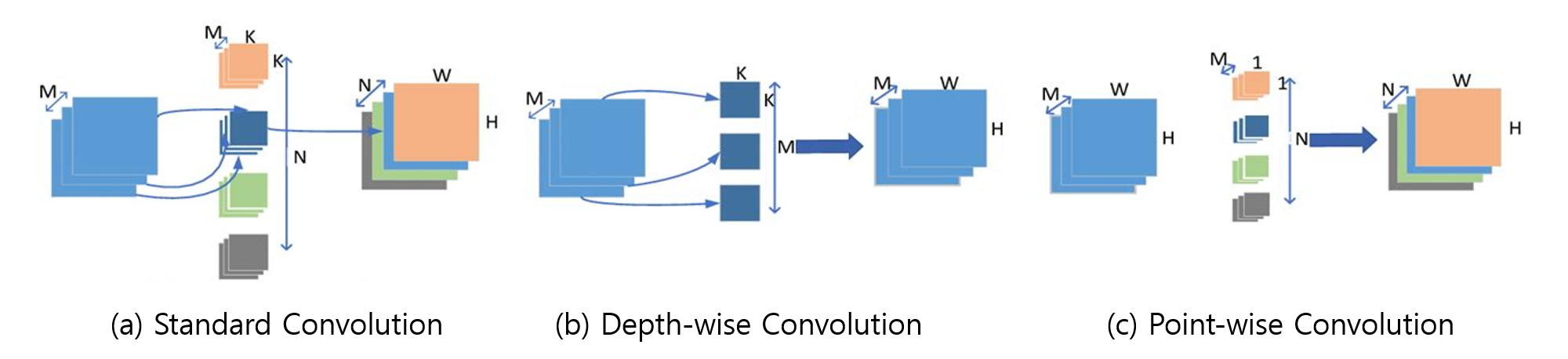
Comparison of Standard vs. Depthwise Separable Convolution: A diagram showing a standard convolution block side-by-side with a depthwise separable block, highlighting the difference in operations and filter dimensions.
4.2 Practical Design Guidelines
When designing a CNN from scratch, choosing hyperparameters is a key challenge. Here are some common practices and starting points:
- Number of Layers (Depth): Start simple and add complexity as needed. A common pattern is to increase the number of filters as the spatial dimensions decrease. For example: 64 filters -> 128 filters -> 256 filters.
- Filter (Kernel) Size: Small filters are preferred. The vast majority of modern CNNs use 3x3 filters. Stacking two 3x3 conv layers has the same effective receptive field as one 5x5 layer but with fewer parameters and more non-linearity. 1x1 filters are also powerful for changing the number of channels (depth).
- Number of Filters (Width): The number of filters in a layer determines the depth of the output feature map. It's common to start with a smaller number (e.g., 32 or 64) in the early layers and progressively increase it in deeper layers. This is because early layers capture simple, universal features, while later layers need more capacity to capture complex, task-specific features.
5. The Training Process
Training a CNN involves more than just feeding it data. It's an iterative process of finding the optimal model parameters (weights) by minimizing a loss function. This requires a combination of core optimization principles and advanced techniques to ensure stable and effective learning.
5.1 The Core Optimization Loop
The training process for a CNN is fundamentally the same as for an MLP. At its heart is a loop that repeats three steps:
- Forward Pass & Loss Calculation: A batch of data is passed through the network to generate predictions. A loss function (e.g., Cross-Entropy for classification) measures the discrepancy between these predictions and the true labels.
- Backward Pass (Backpropagation): The gradient of the loss with respect to every weight in the network is calculated by propagating the error backward from the output layer to the input layer.
- Weight Update: An optimization algorithm (e.g., SGD, Adam) uses these gradients to update the weights, taking a small step in the direction that minimizes the loss.
5.2 Key Strategies for Robust Training
To achieve good performance, several other strategies are employed during training.
Data Augmentation
One of the most effective ways to combat overfitting and improve model generalization is to artificially expand the training dataset. Data augmentation creates modified copies of the training images on-the-fly. For each image, random transformations are applied, such as:
- Random rotations, horizontal/vertical flips, and cropping.
- Changes in brightness, contrast, or saturation.
- Adding small amounts of noise.
This teaches the model to be invariant to these transformations, forcing it to learn the true underlying features of the objects rather than memorizing specific pixel patterns.

Data Augmentation Pipeline Diagram: An illustration showing an original image of a cat being fed into a pipeline that produces several randomly transformed versions (rotated, cropped, flipped, color-shifted) for training.
Learning Rate Scheduling
The learning rate is arguably the most important hyperparameter in training a deep network. A learning rate that is too high can cause the model to diverge, while one that is too low can lead to painfully slow training. Instead of using a fixed learning rate, it's common to use a learning rate scheduler that adjusts the rate during training. Common strategies include:
- Step Decay: The learning rate is reduced by a factor (e.g., by 10) at specific epochs. This allows for large, quick progress at the beginning and finer adjustments as the model converges.
- Cosine Annealing: The learning rate is smoothly decreased from an initial value to a minimum value following a cosine curve. This can lead to better convergence in complex loss landscapes.
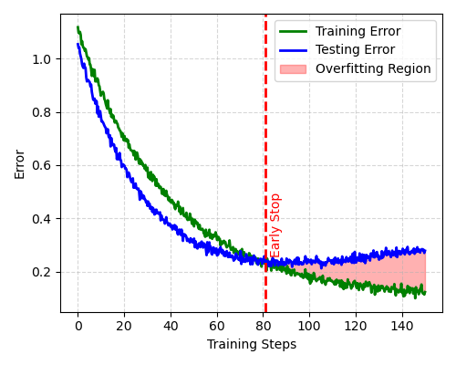
Example Loss Curve for Early Stopping: A graph showing the training loss (continuously decreasing) and the validation loss (decreasing then starting to increase). An arrow points to the minimum of the validation loss curve, indicating the optimal point to stop training.
Regularization to Prevent Overfitting
In addition to Dropout and Batch Normalization (discussed in Section 3), other regularization techniques are vital:
- L2 Regularization (Weight Decay): This technique adds a penalty to the loss function proportional to the squared magnitude of the model's weights. This encourages the network to use smaller, more diffuse weight values, leading to a simpler model that is less likely to overfit.
- Early Stopping: The model's performance on a separate validation set is monitored during training. If the validation loss stops improving (or starts to increase) for a certain number of epochs (the "patience"), the training is halted. The model weights from the point of best validation performance are then saved. This is a simple and highly effective way to prevent the model from overfitting to the training data.
6. Practical Implementation with TensorFlow/Keras
Here's how to build and train a simple CNN for classifying the CIFAR-10 dataset, which contains 60,000 32x32 color images in 10 classes.
import tensorflow as tf
from tensorflow.keras import layers, models
from tensorflow.keras.datasets import cifar10

# 1. Load and normalize the CIFAR-10 dataset
(x_train, y_train), (x_test, y_test) = cifar10.load_data()
x_train = x_train.astype("float32") / 255.0
x_test = x_test.astype("float32") / 255.0

# 2. Define a simple CNN
model = models.Sequential([
    layers.Input(shape=(32, 32, 3)),
    layers.Conv2D(32, (3, 3), padding="same", activation="relu"),
    layers.MaxPooling2D((2, 2)),

    layers.Conv2D(64, (3, 3), padding="same", activation="relu"),
    layers.MaxPooling2D((2, 2)),

    layers.Conv2D(128, (3, 3), padding="same", activation="relu"),
    layers.Flatten(),
    layers.Dense(128, activation="relu"),
    layers.Dropout(0.3),
    layers.Dense(10, activation="softmax")
])

# 3. Compile the model
model.compile(
    optimizer="adam",
    loss="sparse_categorical_crossentropy",
    metrics=["accuracy"]
)

# 4. Train the model
history = model.fit(
    x_train,
    y_train,
    epochs=10,
    batch_size=64,
    validation_split=0.1,
    verbose=1
)

# 5. Evaluate the model
test_loss, test_acc = model.evaluate(x_test, y_test, verbose=0)
print(f"Test accuracy: {test_acc:.4f}")

# 6. Predict a few samples
class_names = [
    "airplane", "automobile", "bird", "cat", "deer",
    "dog", "frog", "horse", "ship", "truck"
]

predictions = model.predict(x_test[:5], verbose=0)
for i, pred in enumerate(predictions):
    predicted_label = class_names[pred.argmax()]
    true_label = class_names[int(y_test[i])]
    print(f"Sample {i}: predicted = {predicted_label}, true = {true_label}")
7. Lab: Classifying CV Data as Images
While an MLP can classify Cyclic Voltammetry (CV) data as a 1D sequence, a CNN can often achieve better performance by treating the data as a 2D representation. This allows the model to learn spatial features from the CV curve's shape, similar to how it learns from an image.
Approach: We will convert each 1D CV curve into a simple 2D black-and-white image. The network will then learn to classify these images. This approach leverages the CNN's ability to recognize shapes, such as the position and form of oxidation and reduction peaks.
import numpy as np
import matplotlib.pyplot as plt
from io import BytesIO
from PIL import Image

import tensorflow as tf
from tensorflow.keras import layers, models
from sklearn.model_selection import train_test_split

# ------------------------------------------------------------
# 1. Generate simple synthetic CV curves for two classes
#    class 0: oxidation peak near +0.25 V
#    class 1: oxidation peak near -0.15 V
# ------------------------------------------------------------
def gaussian(x, mu, sigma, amp):
    return amp * np.exp(-0.5 * ((x - mu) / sigma) ** 2)


def generate_cv_curve(label, n_points=300, noise_level=0.015):
    forward_v = np.linspace(-0.8, 0.8, n_points)
    reverse_v = np.linspace(0.8, -0.8, n_points)

    if label == 0:
        forward_i = gaussian(forward_v, 0.25, 0.11, 1.0)
        reverse_i = -gaussian(reverse_v, 0.10, 0.13, 0.8)
    else:
        forward_i = gaussian(forward_v, -0.15, 0.09, 0.9)
        reverse_i = -gaussian(reverse_v, -0.30, 0.12, 0.75)

    background_f = 0.08 * forward_v
    background_r = 0.08 * reverse_v

    forward_i = forward_i + background_f + np.random.normal(0, noise_level, n_points)
    reverse_i = reverse_i + background_r + np.random.normal(0, noise_level, n_points)

    voltage = np.concatenate([forward_v, reverse_v])
    current = np.concatenate([forward_i, reverse_i])
    return voltage, current


# ------------------------------------------------------------
# 2. Convert each CV curve into a grayscale image
# ------------------------------------------------------------
def cv_to_image(voltage, current, image_size=(96, 96)):
    fig, ax = plt.subplots(figsize=(2.4, 2.4), dpi=40)
    ax.plot(voltage, current, color="black", linewidth=2)
    ax.set_xlim(-0.85, 0.85)
    ax.set_ylim(-1.2, 1.2)
    ax.axis("off")
    fig.tight_layout(pad=0)

    buffer = BytesIO()
    fig.savefig(buffer, format="png", bbox_inches="tight", pad_inches=0)
    plt.close(fig)
    buffer.seek(0)

    image = Image.open(buffer).convert("L")
    image = image.resize(image_size)
    image = np.array(image, dtype=np.float32) / 255.0
    image = 1.0 - image  # black curve on white background -> bright curve on dark background
    return image


# ------------------------------------------------------------
# 3. Build dataset
# ------------------------------------------------------------
images = []
labels = []

n_samples_per_class = 400
for label in [0, 1]:
    for _ in range(n_samples_per_class):
        v, i = generate_cv_curve(label)
        img = cv_to_image(v, i)
        images.append(img)
        labels.append(label)

X = np.array(images)[..., np.newaxis]   # shape: (N, 96, 96, 1)
y = np.array(labels)

X_train, X_test, y_train, y_test = train_test_split(
    X, y, test_size=0.2, random_state=42, stratify=y
)

print("Training set:", X_train.shape, y_train.shape)
print("Test set:", X_test.shape, y_test.shape)


# ------------------------------------------------------------
# 4. Define CNN model
# ------------------------------------------------------------
model = models.Sequential([
    layers.Input(shape=(96, 96, 1)),
    layers.Conv2D(16, (3, 3), activation="relu", padding="same"),
    layers.MaxPooling2D((2, 2)),

    layers.Conv2D(32, (3, 3), activation="relu", padding="same"),
    layers.MaxPooling2D((2, 2)),

    layers.Conv2D(64, (3, 3), activation="relu", padding="same"),
    layers.MaxPooling2D((2, 2)),

    layers.Flatten(),
    layers.Dense(64, activation="relu"),
    layers.Dropout(0.3),
    layers.Dense(2, activation="softmax")
])

model.compile(
    optimizer="adam",
    loss="sparse_categorical_crossentropy",
    metrics=["accuracy"]
)

model.summary()


# ------------------------------------------------------------
# 5. Train and evaluate
# ------------------------------------------------------------
history = model.fit(
    X_train,
    y_train,
    epochs=8,
    batch_size=32,
    validation_split=0.1,
    verbose=1
)

loss, acc = model.evaluate(X_test, y_test, verbose=0)
print(f"Test accuracy: {acc:.4f}")


# ------------------------------------------------------------
# 6. Visualize a few test predictions
# ------------------------------------------------------------
class_names = ["Peak near +0.25 V", "Peak near -0.15 V"]
preds = model.predict(X_test[:6], verbose=0)

fig, axes = plt.subplots(2, 3, figsize=(8, 5))
for ax, image, pred, true_label in zip(axes.ravel(), X_test[:6], preds, y_test[:6]):
    ax.imshow(image.squeeze(), cmap="gray")
    ax.set_title(
        f"Pred: {class_names[pred.argmax()]}\nTrue: {class_names[true_label]}",
        fontsize=9
    )
    ax.axis("off")

plt.tight_layout()
plt.show()
8. Conclusion and Next Steps
Convolutional Neural Networks represent a powerful paradigm for processing structured data with spatial relationships. Their ability to learn hierarchical features through convolutional and pooling operations makes them particularly well-suited for image analysis and other grid-like data structures.
Key takeaways from this guide:
- CNNs use parameter sharing through convolutional filters to efficiently process large input data.
- The combination of convolutional and pooling layers enables the network to learn increasingly complex features.
- CNNs can be adapted for various data types by treating them as 2D representations, as demonstrated in the CV classification lab.
- Modern CNN architectures continue to evolve with techniques like residual connections, attention mechanisms, and efficient attention variants.
As you explore more advanced applications, consider investigating transfer learning with pre-trained models, attention mechanisms in vision transformers, and efficient CNN variants for real-time applications.